GENERAL CHEMISTRY TOPICS

Measurement and units

The International System (SI) of units of measurement. Reliability of measurement. Precision and accuracy, and types of error in measurement. Dimensional analysis. Unit conversions.

---

Measurement is absolutely essential to experimental science. In making a measurement, in a quantitative comparison is being made to some standard that has been adopted for the quantity being measured. An instrument for measurement is calibrated according to the standard, which provides a unit of measurement for that quantity. For instance, in measuring length, a ruler is used which is calibrated in centimeters or inches - both of these are standard lengths or units of length.

Science is an international enterprise, and by consensus the worldwide scientific community has agreed to use a common system of units of measurement of quantities. This International System of Units (Système Internationale d'Unités, abbreviated SI) sets standard units for fundamental physical quantities (such as mass, length, time), as well as for derived physical quantities (labeled as such since they are derived from the fundamental quantities; examples are volume, speed, force).

As foundational to the scientific method as measurement is, so too is the concern with the reliability of any given measurement. In practice, there is error associated with any measurement - that is, the measured value differs from a theoretical true or actual value. Obviously, we seek to minimize error in measurement and obtain a value that is as close to the true value as practical or possible. There are two types of error that we distinguish - random error and systematic error - and these can be related to the specific meanings for the terms accuracy and precision. When we report the result of a measurement, we also report an estimate of the error or uncertainty of the measurement as a matter of good scientific practice. The number of significant figures for a reported measurement is directly related to the decimal place where the uncertainty of the measurement no longer allows us to say with complete confidence what the digit in that place should be in order to correspond to the true value of what we are trying to measure. There are sophisticated statistical methods to help scientists detect the presence of error, and to deal with propagation of error in calculations. In a first general chemistry course, we will not consider such methods, instead settling for a understanding of significant figures and some rules of thumb for treating them in calculations.

Precision and accuracy, and types of error

These terms have very (pardon the pun) precise meanings for the working scientist, despite their being roughly synonymous in everyday use. The shorthand definitions:

• Precision = reproducibility of a measurement
• Accuracy = closeness of measurement to "true" value

The types of experimental error are related to this distinction. Random error is inherent in any experimental measurement, and is reflected in the precision of the measurement (less random error = more precision). Superimposed on random error may be systematic error - the measurement is reproducibly off, or inaccurate, - if the method of making the measurement is flawed.

Accuracy and precision

Any time measurements are performed in scientific investigations, errors or a degree of uncertainty in these measurements are possible, and indeed, inevitable. The measured value may be close to or far from the true value of what is being measured. Our only hope to identify and take account of errors in measurement is to perform repeated, or replicate measurements using a particular method or technique, and to do the same (if possible) with a different method or independent technique. Then it is at least possible to analyze the statistics of data obtained from our measurements.

There are two qualitatively different ways in which the reliability of measurement is characterized in scientific investigations. Accuracy refers to closeness of the measurements to the true value, and precision refers to the reproducibility, or consistency, of the measurements. A helpful way to represent these ideas pictorially is to think of replicate measurements as shots at a target by a particular marksman at a rifle range, and different marksmen (or markswomen) representing different "methods" of measurement. The target bull's-eye is the true value of the measurement. Consider then the following results of four different methods for hitting the target:

 

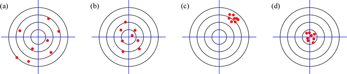
In a basic statistical treatment of the results of replicate measurements by a given method, we would calculate the average value and the standard deviation. In (a), the shots are widely scattered (which would produce a large standard deviation) and this is what we would call low precision. Furthermore the average value of the shots is off-target (it appears to be somewhere to the southwest of the bull's-eye) and this is what we would call low accuracy or inaccurate. In (b), there is somewhat less scatter, so precision is improved over (a), and the average looks closer to the center of the target, so accuracy has improved as well. In (c), we see a great improvement in precision (the shots are highly reproducible), but the average is clearly way off the mark. This marksmanship is precise, but inaccurate. Finally, in (d), we see the combination of high accuracy and good precision. The standard deviation of these shots is relatively small, and their average value is quite close to the true value.

With this illustration of accuracy and precision in mind, let us revisit the concepts of random error and systematic error, and see how these types of experimental error are related to this distinction. Random error inherent in any experimental measurement is reflected in the precision of the measurement (less random error = more precision). Superimposed on random error may be systematic error - the measurement is reproducibly off-target, or inaccurate, - if the method of making the measurement is flawed. Reinterpreting the target diagram above, (a) shows the greatest degree of random error, with (b) showing somewhat less. Both (c) and (d) reflect low random error. However, systematic error is most evident in (c), as the average of location of the shots (the measurements) is far from the bulls-eye (the true value that the measurements are "aimed" for). The shots in (a) are the result of significant systematic and random error.

The SI system and units of measurement

When we begin to apply scientific measurement to the universe around us, certain quantities suggest themselves as fundamental in nature. Those relating to space and time seem a priori fundamental, as does the quantity mass, which is a property of all matter. Other quantities might be considered fundamental because they are simply and accurately measurable. The set of fundamental quantities are chosen so that measurement of any other quantifiable property can be made in terms of units derived from this basic set. These fundamental quantities, defined as part of the SI system, are mass (M), length (L), time (T), chemical amount (n), temperature (t), electric current (I), and luminous intensity.

Quantities such as area (L²), volume (L³), speed (L·T⁻¹), acceleration, force, pressure, energy, etc. have been given SI units that are derived from the SI base, or fundamental units. Table 1 below summarizes base SI units. Table 2 lists the common decimal multipliers with their prefixes.

	Table 1: Fundamental units
	Quantity	SI Unit	Notes
	Mass	kilogram (kg)	Pt/Ir bar in vault in Paris*
	Length	meter (m)	light travels this far in 1/299,792,458 s
	Time	second (s)	based on a specific electronic transition frequency of 133Cs
	Chemical amount	mole (mol)	6.022142 × 1023 mol−1 conversion factor
	Temperature	kelvin (K)	absolute temperature scale; for ΔT, 1 K = 1 °C
	Electric current	ampere (A)	used to derive the Coulomb (C), SI unit for electric charge
	luminous intensity	candela (cd)
	For further information, see the SI Section of Ref.3, and also Ref.6. * Recently the kg was redefined - see Ref.5 for a report

	Table 2: Decimal multipliers
	prefix	multiplier		prefix	multiplier
	deka (da)	101		deci (d)	10−1
	hecto (h)	102		centi (c)	10−2
	kilo (k)	103		milli (m)	10−3
	mega (M)	106		micro (µ)	10−6
	giga (G)	109		nano (n)	10−9
	tera (T)	1012		pico (p)	10−12
	peta (P)	1015		femto (f)	10−15
	exa (E)	1018		atto (a)	10−18

Dimensional analysis, unit conversions

Dimensional analysis of a calculation simply means that we treat the units in a calculation algebraically - when we multiply or divide terms, we do the same with the units. In a ratio, common factors cancel. When adding or subtracting terms, those terms must be expressed in the same units, otherwise you are adding together apples and oranges, i.e. you can't sensibly add/subtract those numbers. When setting up and performing any calculation where numbers or measurements with units are involved, one should always check whether the dimensional analysis of the calculation yields the correct units. Arguments to functions such as log and exp should be dimensionless. Often, looking at the units can guide you in what calculation to perform. If the dimensional analysis of a calculation shows the correct units are produced, it does not guarantee the calculation is correct. However, if the dimensional analysis of a calculation shows that it yields the wrong units, the calculation is certainly wrong.

Always include units in writing out the calculations you perform. This will help you avoid many mistakes and help give your instructor at least the impression you know what you are doing!

Any definition of units of a quantity provides a(n exact) conversion factor. For example, the definition

1 in = 2.54 cm exactly

expresses an equivalence relation between length quantities expressed in units inches (in) to the same quantities in units centimeters (cm). This equivalence relation gives rise to the conversion factor 2.54 cm/in. In this instance, the conversion is exact (no loss of significant figures). So to convert inches to centimeters, we need a conversion factor of cm/in to multiply the length quantity in inches.

(6.3360 × 10⁵ in ) (2.54 cm·in⁻¹) = 2.4945 × 10⁵ cm

For the opposite conversion, centimeters to inches, the inverse factor, in/cm, is applied as follows

30.50 cm (2.54 cm·in⁻¹)⁻¹ = 12.01 in

The decimal multipliers work similarly to exact conversion factors. If, for example, we needed to convert between meters (m) and nanometers (nm), we recognize that

(x nm ) (10⁻⁹ m·nm⁻¹) = y m
(y m ) (10⁹ nm·m⁻¹) = x nm

and the decimal multiplier conversion factor does not affect the number of significant figures.

For more examples, see Conversions and dimensional analysis topics page.