GENERAL CHEMISTRY TOPICS
The quantum-mechanical atom
Conundrums of the early 20th century. Paradoxes of the Rutherford model. Quantum mechanics and the atom. Orbitals for the hydrogen atom. Size, shape, and orientation of the orbitals. Electron configurations. Experimental verification of electron configurations.
Rutherford's nuclear model of the atom
At the beginning of the 20th century, the nature of the atom came to be addressed with increasing interest by the greatest scientific minds of the time as discoveries began to reveal the existence of even more minute entities contained within. A key discovery, due to the work of J. J. Thomson, that cathode rays were beams of tiny negatively-charged particles, called electrons, and that all atoms contained these electrons, led to his proposal of a rather whimsically named "plum pudding" model. In this model, electrons were envisioned as embedded like raisins in an amorphous, spherical distribution of positively-charged pudding. In 1910 Ernest Rutherford, who had been a student of Thomson's, and associates performed experiments that blew up the plum pudding model. A beam of α (alpha) particles was aimed at a very thin piece of gold foil. Most of the α particles (which are 4He nuclei) passed right through the foil. A few were deflected through small angles. Only a very few (about 1 in 20,000) were scattered through angles greater than 90° as if they had encountered something massive that scattered these very few α particles backward. The interpretation of these results was that most of the mass and positive charge of the gold atoms was concentrated in a nucleus - at the center of the atoms in a very small volume relative to their apparent size. Rutherford was able to calculate that the radius of the nucleus was at least 10,000 times smaller than the atomic radius. The Rutherford model was a nuclear model of the atom, but not much could be said about electrons. Although they carry all the negative charge of an atom, electrons account for only a tiny fraction of its mass (an electron is about four orders of magnitude, or 104 times, smaller than a proton). What would take the place of the plum pudding model? If most of the mass and positive charge of the atom was concentrated in a nucleus, it seemed all too natural to propose a planetary model for the electrons in an atom, whirling about the nuclear sun in orbits. Especially so in view of the fact that both gravitational and electric attractive force follow an inverse-square law. In Rutherford's new planetary model of the atom, electron orbits distributed around the nucleus would define the size of the atom, but overall, most of the atomic volume was simply empty space. Contradictions within this planetary model would soon become apparent.
Paradoxes of the planetary model
Questions arising from Rutherford's model of the atom concerned the stability of atoms. Leaving aside the question of how so many protons could be forced together into the tiny nuclear volume of a heavy atom, consider the simplest case, a hydrogen atom. The law of electrostatic potential energy (see the energy webpage) shows that for an electron in the neighborhood of a proton, the potential energy of the attraction between them is proportional to −1/r, where r is the distance of separation. The closer the electron and proton are to one another, the more negative the potential energy becomes. This alone would tend to draw the electron and proton together to lower the energy of the two-particle system, and lead to the collapse of the atom. Yet electrons in atoms occupy a relatively vast region of space outside the nucleus. How do the electron and nucleus remain a safe distance apart? Electrons must be moving within the atomic volume - how else could such a relatively small particle seemingly occupy so much space? If the electron, which as a particle has mass, is moving, it has kinetic energy as well. One possibility is that like a planet in the solar system, the kinetic energy of an electron keeps it in a stable trajectory or orbit around the nucleus. If the internal energy of the atom is conserved, if the electron lost potential energy by approaching the nucleus more closely, it would gain kinetic energy. The increased velocity would tend to move the electron further away from the nucleus. The idea that electrons move in trajectories, analogously to planets in orbits was a characteristic feature of the Bohr model of the atom, proposed in 1913 by the great Danish physicist Niels Bohr along with Rutherford.
The Bohr model was an intriguing advance since it restricted the electron in a hydrogen atom to specific radii, and the associated energies accounted for the hydrogen emission spectrum. Despite this success, the Bohr model still suffered from critical defects. For one, treating the electron strictly as a particle - in the classical sense, with a trajectory defined by its position and momentum through time - conflicted with the theory of classical electrodynamics. The latter predicted that as a charged particle, an electron moving in an orbit would continuously lose energy by emitting electromagnetic radiation. Furthermore, the "quantized" energy levels of the Bohr model did not arise from any underlying principle or theoretical understanding of the atom. The paradox of atomic stability could not be fully resolved until the advent of quantum mechanics in the 1920s.
Quantum mechanics and the atom
The particle-like nature of EM radiation has its counterpart in the nature of particles at the atomic and sub-atomic scale. This brilliant insight was produced by French physicist Louis de Broglie in 1924, who proposed that the wavelength of a particle was inversely proportional to its (scalar) momentum. The proportionality constant is Planck's constant, the very same constant relating EM radiation frequency to energy.
Once the wave-like nature of particles was applied to an electron within the atom (as first demonstrated by Erwin Schrödinger in 1927), not only were the paradoxes of the atom that emerged at the dawn of the 20th century resolved, but the quantized nature of electron energies arose naturally - as opposed to the rather ad hoc supposition of the Bohr model. In place of the Bohr model, a profoundly different view of the atom emerged.
A guitar string, or generally speaking, a vibrating string with two fixed end points serves as a
one-dimensional analogy to the treatment of an electron bound to a nucleus
by the electrostatic force of attraction as a three-dimensional "electron-wave".
A mathematical description of a guitar string with fixed length L is a "wave" equation
with a set of solutions, or "wave" functions.
Such wave functions must satisfy the boundary conditions that the amplitude is zero
at both ends of the string. Placing the string on a horizontal "x" axis with one
end at x = 0 and the other at x = L, the amplitude must always be zero
at these two end points. These conditions allow a series of standing wave solutions
in which an integral number of half-wavelengths matching L exactly. The
figure (below, right) illustrates the guitar string wave functions for one, two,
and three half-wavelengths.
The following equation expresses the general condition on wavelength λ:
½nλ = L, where n = 1, 2, 3, ...
This can be rearranged as
λ = 2L/n, where n = 1, 2, 3, ...
which shows that a sinusoidal standing wave function for a one-dimensional guitar string is restricted to a set of discrete wavelengths.
Beyond the first guitar string wave function (with n = 1 and the longest wavelength) there are one or more points along the vibrating string where its amplitude remains at zero. Such points are called nodes, and we will see similar nodal features for electron probability amplitudes in atoms. For now we note that for the one-dimensional vibrating string, a wave function characterized by what we can call a quantum number, here corresponding to the value of the positive integer n, there are n − 1 nodes.
For the electron in an atom, the analogous wave equation solutions (wave functions, Ψ) are three-dimensional and rather than a single quantum number n, these solutions are specified by a set of three quantum numbers: n, the principal quantum number; l, the angular momentum quantum number; and ml, the magnetic quantum number (see below). We can think of the quantum numbers as labels, or indices, of the solutions to the Schrödinger equation, and also note that each solution (we'll call these solutions orbitals) is associated with a definite energy E.
The Schrödinger equation, HΨ = EΨ merits further description. Interpreting this equation term by term, H stands for Hamiltonian, and is a type of operator. An operator is a function that takes another function as an input, and "operates" on it, thereby converting it to an output function. The Hamiltonian includes terms for the kinetic and potential energy of a particle. The particle will be represented by its wave function Ψ, and when the operator acts upon the wave function, the equation says that the output wave function will be the same as the input wave function, except for its being multiplied by a numerical factor. This scalar quantity is the energy E of the particle, specifically the energy that matches its description by the wave function. When a wave function satisfies this condition, it it said to be a solution to the Schrödinger equation. It turns out for the case of a single electron bound its nucleus (such as 1H, 2H, 3H, 4He+), there are multiple solutions corresponding to the discrete, or quantized energies that account for the observed emission spectra of one-electron species, just like the Bohr model. Quite unlike the Bohr model however, the electron is not travelling in a trajectory or orbit, but is being described as a wave function.
Although the wave function Ψ has no direct physical interpretation, its square (Ψ2) is a probability distribution function that describes the probability of finding the electron in any given location relative to the nucleus.
Orbitals for the hydrogen atom
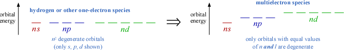
The rules for quantum numbers define the sets of orbitals possible for an electron bound to a nucleus. There are n2 orbitals for any given value of the principal quantum number n. In the case of the hydrogen atom, the energies are determined only by the principal quantum number n, and all n2 orbitals for a given n are all equal in energy (and are therefore termed degenerate). The energy level diagram for electronic orbitals in the hydrogen shown below. In this diagram, we introduce the chemistry convention for naming orbitals according to their set of quantum numbers. The principal quantum number n is retained, while the angular momentum quantum number l is replaced with a set of letter designations (s, p, d, ...).
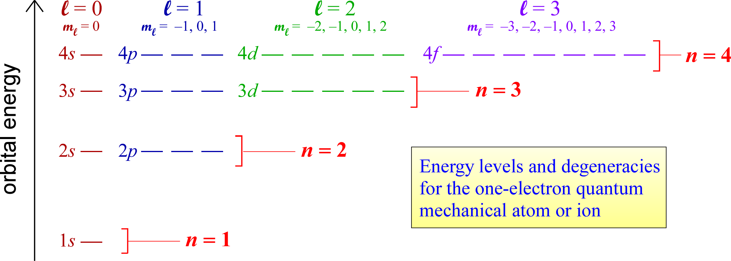
The distinct energy levels for a hydrogen atom and orbital degeneracies suggest that we can think of groups of degenerate orbitals as organizing electrons in many-electron species into energy-level "shells" that at first glance correspond to seperate values of the principal quantum number n.
Size, shape, and orientation of the orbitals
The shapes of the orbitals are determined by the angular momentum quantum number l. The orbitals for which l = 0 are spherically symmetric around the nucleus, and are labeled as s orbitals. For l = 1, a set of three mutually perpendicular dumbbell-shaped p orbitals arise. When l = 2, five so-called d orbitals with more complex shapes are possible. The orientations of the p- and d- and all higher l value orbitals are specified by the magnetic quantum number ml. For further exploration of the sizes, shapes, orientations, and other features such as radial distribution functions, a trip to The Orbitron is highly recommended. Be sure to check out the exotic shapes of f and g orbitals!
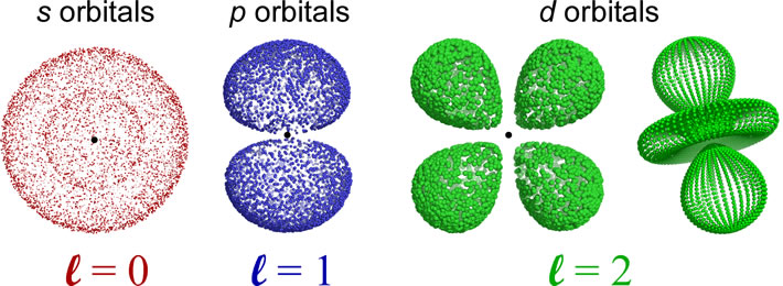
Nodes: An orbital will have n − 1 total nodes, with n − l − 1 radial nodes, and l angular nodes. The s orbital depicted is a 2s orbital, and the single node is a radial node. There are no angular nodes in any s-type orbital, since l = 0 for any s orbital. The p orbital depicted is a 2p orbital, which also has a single node, which is an angular node - in this case the plane containing the nucleus and bisecting the two lobes of the p orbital. There are two different 3d orbitals depicted - both have two angular nodes and zero radial nodes.
Multielectron atoms
The quantum mechanical model for the hydrogen atom was a spectacular success. It accounted for the hydrogen emission spectrum and yielded a set of exact mathematical equations describing the three-dimensional probability distribution for an electron in an orbital of any of the allowed energy levels. We see represented above the different sizes and shapes of the prime examples of these probability distributions, and their association with specific sets of quantum numbers, along with the letter labels for the values of the angular momentum quantum number l, the chemistry notation. How does the quantum mechanical model work with all the other atoms beyond hydrogen? Are the same orbital shapes valid? How do electrons occupy orbitals in these atoms? Can the orbital energies for electrons in multielectron atoms be theoretically determined? What experimental evidence can be used to verify orbital occupancy in multielectron atoms? In what follows on this page, we address these questions.
In the case of the hydrogen atom (and other one-electron species such as He+), the Schrödinger equation can be solved exactly. However, once we have to account for any additional electrons, the Schrödinger equation for such systems becomes unsolvable. This is because the number of potential energy terms (given by Coulomb's Law) rapidly increases.
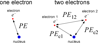
The accompanying figure illustrates this by comparing the Coulombic energy terms for a one-electron and a two-electron species. In the former, treating the nucleus and the electron as point charges, there is only one potential energy term for the attraction between the electron and the nucleus. In the latter case, not only is there an additional attractive term for the interaction between the next electron and the nucleus, but now there is a term for electron-electron repulsion (labeled PE12 in the diagram). The number of repulsive terms to be accounted for increases rapidly with each additional electron added. Of course in the quantum mechanical model, electrons are not treated as particles and orbitals are described by means of wave functions. The Schrödinger equation must still include terms for all potential energies and the resulting equation becomes too complex to solve directly. The good news is that approximate solutions for many-electron atoms using the same orbitals and quantum numbers developed for the hydrogen atom can be obtained that yield predictions about the properties of atoms that agree well with experiment. The principal difference is that orbital energies no longer depend on just n, but on both n and l.
Sublevel energy splitting in multi-electron species
Why do the orbitals of multielectron atoms and monatomic ions have energies that depend on the value of both n and l? This is called sublevel splitting. The principal quantum number n determines the general size of the orbitals, with size increasing with increasing n. We know that larger orbitals have higher energies becuse on average the electron is more likely to be found further from the nucleus than in a smaller (lower value n) orbital. This is shown clearly by comparing the radial distribution functions for 1s, 2s, and 3s orbitals. However, comparing radial distributions of orbitals with different values of l but the same value of n shows that the s orbital penetrates more close to the nucleus, and the p orbital penetrates better than the d orbital, and so on. Because of the way in which electrons occupy orbitals in multielectron atoms and the shapes and sizes of these orbitals, the energies of sublevels are no longer the same for a given value of n, the energies these orbitals are in the order ns < np < nd < ···.
Once a second electron is introduced, the extra electric forces affect the orbital energies. In particular, the energies of electrons in orbitals with the same value of the principal quantum number n but different values of the angular momentum quantum number l become slightly different. Why is this the case? The short answer is that the different shapes of the orbitals lead to their having slightly different energies in the context of the presence of other electrons. To give a more satisfactory answer, we have to dig into the weeds a bit and discuss the matter in terms of these three concepts: Coulomb's Law, shielding, and penetration.
If we consider the two electrons depicted at left as residing in separate orbitals of equal n but different l. For example in boron with 5 electrons, we can focus on two electrons, one occupying a 2s orbital (n = 2, l = 0) and the one occupying a 2p orbital (n = 2, l = 1), the two 1s electrons will be on average significantly closer to the nucleus than the three electrons in the n = 2 shell. Thus not only will these electrons experience greater attraction to nucleus and have lower energy (Coulomb's law), but they will also shield the n = 2 electrons from the full +5 charge of the nucleus. So these electrons are both further on average from the nucleus and experiencing a lowered effective nuclear charge (denoted as Zeff, so we are saying that for the n = 2 electrons, Zeff
So far we have just given a little more nuance to the explanation of the increase in orbital energies with increasing n, but having introduced Coulomb's law, shielding, and Zeff, we can now look at the effect of l on orbital energies in multielectron atoms. To do so, we will need to look more carefully at the probability distributions of the orbitals, and in particular, the radial probability distributions. The radial probability distribution of an orbital shows the probability of finding the electron at a distance r from the nucleus.
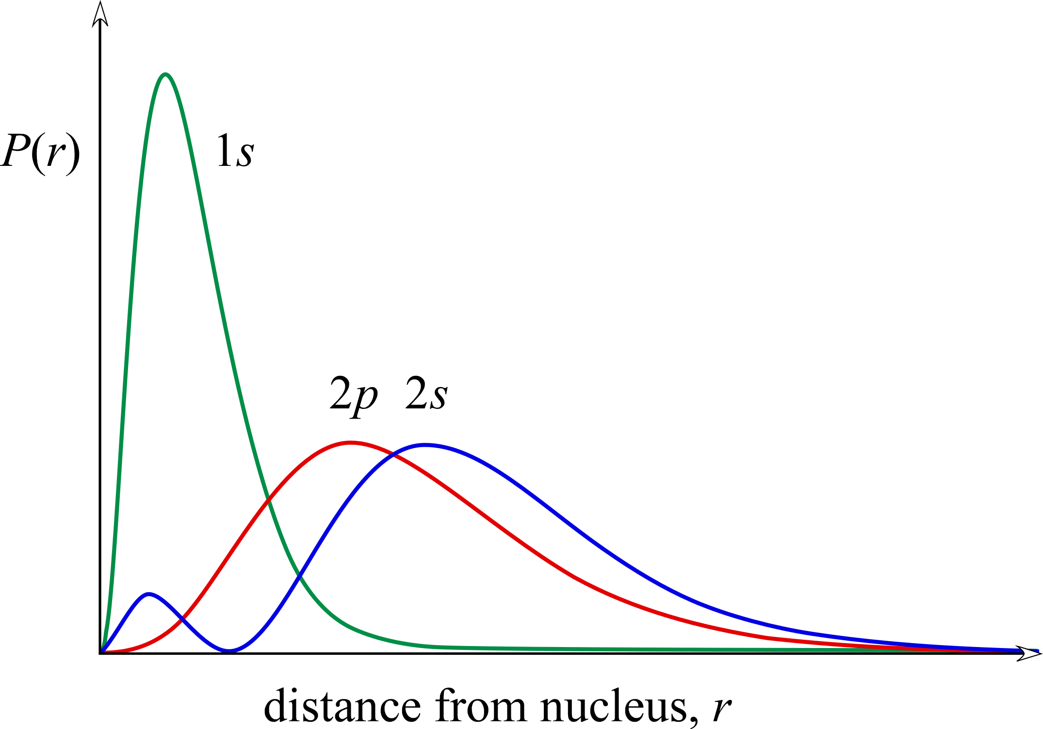
Comparing the radial distributions for 1s, 2s and 2p (see figure below), it is apparent that most of the radial probability for the latter two orbitals lies outside of the bulk of the 1s radial probability. The interesting and relevant features here arise from the comparison of the 2s and 2p orbitals. While the 2p orbital has a radial probability density maximum at a value of r less than that of the 2s orbital, the 2s orbital penetrates closer to the nucleus with its minor peak within the sphere defined by its radial node (at the value of r for which the probability of finding the electron goes to zero). The extra penetration of the 2s orbital into the inner portion of the 1s orbital distribution is responsible for the lower energy of a 2s electron compared to the 2p electron. We can say that this penetration of a 2s electron outweighs the lesser penetration of the 2p electron, as well as the occurrence of the 2p maximum radial probability at a closer distance r from the nucleus, so that Zeff is greater for the 2s electron than it is for the 2p electron. The 2p electron is more shielded from the full nuclear charge Z than is the 2s electron.
When we get to n = 3 and consider as well the d subshell orbitals, the situation is similar. Since the penetration of 3s orbital is greater than that of the 3p orbital, and greater still than the 3d orbital, an electron in a 3s experiences the greatest Zeff, hence the lowest energy of electrons in any n = 3 orbital. Electrons in 3p orbitals are a little higher in energy than 3s electrons, while the further increase in energy for 3d electrons makes thier energies comparable to the those for lowest energy subshell for the next value of n, the 4s orbital. The latter is in fact is filled before the 3d orbital as we build up electron configurations for elements beyond Period 2.
Electron configurations and their experimental verification
Electron configurations tell us how electrons are distributed within atoms. This essentially quantum-mechanical description of atoms provides the underlying explanation of the chemical properties of the elements. In particular, the energy levels available to and "occupied" by electrons in all the various atoms that make up the elements explain the structure and organization of the periodic table. The quantum model for the atom must account for all relevant experimental observations, and for the electrons, our predictions from the quantum mechanical theory must accord with observable properties, such as absorption or emission spectra.
As a brief introduction to the quantum mechanical rules for how electrons occupy orbitals in atoms and how these electron configurations are represented, consider the electron to be represented as a vertical single-barbed arrow. Starting with hydrogen, a single electron will normally occupy the orbital of lowest energy available, which would be the 1s orbital. Symbolically, we can represent this hydrogen atom ground state electron configuration by placing a barbed-arrow at the 1s level in our energy-level diagram. Alternatively, the arrow can be placed in a box labeled "1s". Taking the next step to helium immediately raises the question of whether the lowest energy orbital available is still the 1s. Can the second electron also be described by 1s orbital electron probability distribution function (ψ21s)? The rules of quantum mechanics specify that the quantum distribution of each electron within an atom must be described by its own unique set of quantum numbers.
Paramagnetism. Although electrons do not spin in a literal sense, electrons have magnetic properties in just the same way a spinning charged sphere would have in the macroscopic realm. If in an atomic electron configuration any orbitals are singly occupied, such electrons are said to be unpaired. The presence of unpaired electrons in the atoms that make up a substance render it paramagnetic, meaning it is attracted into a magnetic field. Substances with no unpaired electrons have weaker magnetic properties, and are said to be diamagnetic, and subject to a very weak repulsive force in a magnetic field. Determining whether a pure elemental substance is paramagnetic or diamagnetic doesn't tell us the ground state electron configuration of its atoms, but the configuration we predict by "building-up" as illustrated above had better be consistent with the observed magnetic properties.
Photoelectron spectroscopy (PES). Based on the photoelectric effect, PES allows for a direct measurement of orbital energies. In PES, a gaseous sample of a pure element is illuminated with a beam of EM radiation of a specific frequency with energy is sufficient - when absorbed by an atom - to eject its electrons. The ejected electrons, termed photoelectrons, are detected and their kinetic energies measured. This information yields the binding energy of the electrons in an atom. The results of PES experiments, by showing the number of electrons at each of the allowed energy levels for an atom, indicate the existence of shells and subshells.